Nkululeko: how to plot distributions of feature values

As shown in this post, with Nkululeko you can select only specific features from your features sets by specifying them in the [FEAT] section:

[FEATS]
features = ['JitterPCA', 'meanF0Hz', 'hld_sylRate']

What you can also do, is plotting them per category (only for classification), by specifying in the PLOT section if you would like that for all samples or only test or train samples:

[EXPL]
# turn it on
feature_distributions = True 
# use only training samples
sample_selection = train 
# only plot the 5 most important features 
max_feats = 5  

You would have to call nkululeko with the explore interface:

python -m nkululeko.explore --config <myConfig.ini>

The image file is in the image folder and should look similar to this:

Nkululeko: how to predict many samples

There are three ways to predict a number of samples:

  1. If you want to save the predictions of an experiment for later use, you can do so by stating in the EXP section

    [EXP]
    save_test = ./my_saved_test_predictions.csv

    The output format is CSV, comma seperated values.

  2. Alternatively, you can test an existing database against the best model you trained before, by stating the databases as tests in the DATA section:

    [DATA]
    tests = ['my_testdb']
    my_testdb = /mypath/my_testdb
    ...

    and then calling Nkululeko's test module

    python -m nkululeko.test --config mycoonfg.ini --outfile myresults.csv
  3. Run the demo module simply for a set of files:

    python -m nkululeko.demo --config mycoonfg.ini --list my_filelist.txt

How to normalize features

"Normalizing" or scaling feature values means to shift them to a common range, or distribution with same mean and standard deviation (also called z-transformation).
You would do that for several reasons:

  • Artificial neural nets can handle small numbers best, so they all should be in the range -1, 1
  • Speakers have their individual ways to speak which you are not interested in if you want to learn a general task, e.g. emotion or age. So you would speaker-normalize the values for each speaker individually. Of course this is in most applications not possible because you don't have already samples of your test speakers.
  • You might want to normalize the sexes, because woman typicall have a higher pitch. But another way out is also to use only relative values and not absolute ones.

Mind that you shouldn't use your test set for normalization as it really only should be used for test and is supposed to be unknown. That's why you should compute your normalization parameters on the training set, you can then use them to normalize/scale the test.

Augmenting data

Often (kind of always) there is a lack of training data for supervised learning.

One way to tackle this is representation learning which can be done in an self-supervised fashion.

Another approach is to multiply your labeled training data by adding slightly altered versions of it, that would not change the information that is the aim of the detection, for example by adding noise to the data or clipping it. This is called augmentation and here is a post how to do this with nkululeko.

A third way is to synthesize data based on the labeled training, for example with GANs, VAEs or with rule-based simulation. It can be distinguished if in this case only a parameterized for of the samples (ie. the features) or whole audio files are generated.

Sometimes only samples for a rare class are needed, in this case techniques like ROS (random over sampling), Synthetic Minority Oversampling Technique (SMOTE) or the Adaptive Synthetic (ADASYN) can be used.
Here is a post how to do this with nkululeko

Nkululeko

This is the entry post for Nkululeko: a framework to do machine learning experiments on audio data based on configuration files.

Here's an overview on the tutorials:

Meta parameter tuning

The parameters that configure machine learning algorithms are called meta parameters in contrast to the "normal" parameters that are learned during training.

But as they obviously also influence the quality of your predictions, these parameters also must be learned.

Examples are

  • the C parameter for SVM
  • the number of subsamples for XGB
  • the number of layers and neurons for a neural net

The naive approach is simply to try them all,
how to do this with Nkululeko is described here

But in general, because the search space for the optimal configuration usually is without limit, it'd be better to try a stochastic approach or a genetic one.

How to split your data

In supervised machine learning, you usually need three kinds of data sets:

  • train data: to teach the model the relation between data and labels
  • dev data: (short for development) to tune meta parameters of your model, e.g. number of neurons, batch size or learning rate.
  • test data: to evaluate your model ONCE at the end to check on generalization

Of course all this is to prevent overfitting on your train and/or dev data.

If you've used your test data for a while, you might need to find a new set, as chances are high that you overfitted on your test during experiments.

So what's a good split?

Some rules apply:

  • train and dev can be from the same set, but the test set is ideally from a different database.
  • if you don't have so much data, a 80/20/20 % split is normal
  • if you have masses an data, use only so much dev and test that your population seems covered.
  • If you have really little data: use x cross validation for train and dev, still the test set should be extra

Nkululeko exercise

Edit the demo configuration

1)
Set/keep as target emotion as FEAT type os and as MODEL type xgb

Use the emodb as test and train set but try out all split methods

  • specified
  • speaker split
  • random
  • loso
  • logo
  • 5_fold_cross_validation

Which works best and why?

2)
Set the

[EXP]
epochs = 200
[MODEL] 
type = mlp
layers = {'l1':1024, 'l2':64} 
save = True
[PLOT]
epoch_progression = True
best_model = True

run the experiment.
Find the epoch progression plot and see at which epoch overfitting starts.

How to evaluate your model

This post is about evaluation of machine learning models, obviously the answer to the question if a model is any good depends a lot on how you test that.

Criteria

Depending whether you got a classification or regression problem you can choose from a multitude of measures.

Classification

Most of these are derived from the confusion matrix:

  • Confusion Matrix : Matrix with results: rows represent the real values and columns the predictions. In the binary case, the cells are called True Positive (TP), False Negative (FN: Type 2 error), False Positive (FN: Type 1 error) and True Negative (TN)
    Here's a plot of cases: idea

    In this figure, the circles are the relevant samples and the crosses are the not-relevant ones. Now the relevant ones that are not in the selected area are False Negatives, and the ones inside are True Positive.

And this would be the confusion matrix:

So in the example above, TP=3, FN=4, FP=3 and TN=3.

The following measurements can be derived from these:

  • Accuracy: Percentage of correct predictions -> (TP+TN)/(TP+FP+FN+TN).

  • un- / weighted Recall/Sensitivity: percentage of detected cases -> TP / (TP+FN). Can be weighted by class frequency, for multiple classes

  • un- / weighted Precision: percentage of relevant predictions -> TP / (TP+FP)

  • Specificity: Like sensitivity, but for the negative examples -> TN / (TN+FP)

  • F1: Combination of Recall and Precision -> F1 = 2 (Rec Prec)/ (Rec + Prec)

  • AUC/ROC Usually there's a tradeoff between Recall and Precision. With the Receiver Operator Curve and it's Area under curve this can be visualized by plotting the False positive rate (100-specificity) against the True positive rate (sensitivity).

    Regression

  • Pearson's Pearson's Correlation Coefficient measures the similarity of two sets of numbers with the same lenght. I's a value between -1 and 1, with 0 meaning no correlation and -1 negative correlation. When plotted in 2-d space, PCC=1 would be the identity line.

  • MAE Mean absolute error: taken two sets of numbers with same length as correct and predicted values, one can compute the mean absolute error by summing up the absolute values of the pairwise differences and scale by the number of samples.

  • CCC Concordance Correlation Coefficient is a measure quite similar to PCC but tries to penalize rater bias (seeing the two distributions as truth and ratings).

Approaches

Train / test /dev splits

Best you have enough data to split it into seperate sets:

  • train for the training
  • dev to tune meta-parameters
  • test as a final test set

Be careful to make sure that they are speaker disjunct, i.e. not have overlapping speakers, else you can't be sure if you learn general speaker characteristics or speaker idiosyncrasies.

Also it's a very good idea to have the test set from a completely different data source, so you could have more trust in the generalizability of your model.

More on the subject here

X fold cross validation

If you are low on data, you might try x fold cross validation, it means that you split your data in x (usually 10) sets with same size, and then do x trainings, using one set as dev set and the rest for train.

LOSO

Leave one Speaker out is like X fold cross-validation, but each set are all samples of one speaker. If there are many speakers, you might want Leave one speaker group out.
Both is supported by Nkululeko.

Different machine learners

This post gives an overview on popular machine learners in a nutshell.
Lots of site on the internet give great detail on this and you should take a few minuted to check them out.

Preliminaries and some naming conventions

In general, all these approaches work by extracting features from data and comparing a test sample's features with the features derived from a training set to predict some class or value in case of regression.

So they work with two phases:

  • During training, the parameters of the approach are learned, thereby creating the model.
  • A test time, unknown test samples get predicted by the model.

In addition, most of these approaches can be customized by meta-parameters which also can be learned by some meta algorithm, but not during a normal training.

One thing all of these approaches have in common is that they model the world by "densing" down the real values, i.e. the data, to a simpler form at some time (feature extraction), so they all can be seen as some kind of dimensionality reduction

On the one hand you lose information this way, on the other this is not a problem because you usually are interested in some kind of underlying principle that generated your training data, and not so much in the training data itself.
Still you got a trade-off between generality and specificity

Obviously, the following list is by far not complete, I simply selected the ones that were most commonly used during my professional life.

Linear regression

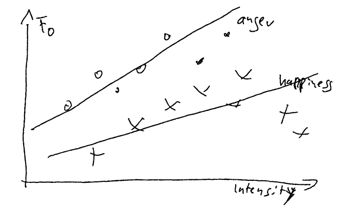
To represent the dependency of a dependend and an independend variable by a straight line. The price question is how to learn the two parameters of the line (a and b of y=ax+b) using the training data. One approach would be gradient descent with a Perceptron.


Fig.: Two linear regression models for anger and happiness based on mean fundamental frequency (F0)

GMMs

A Gaussian is a way to describe a distribution with two values: mean and variance. Now one way to distinguish two kinds of things is two distinguish them by the distributions of their features, e.g. herrings from trouts by the size of their fins.
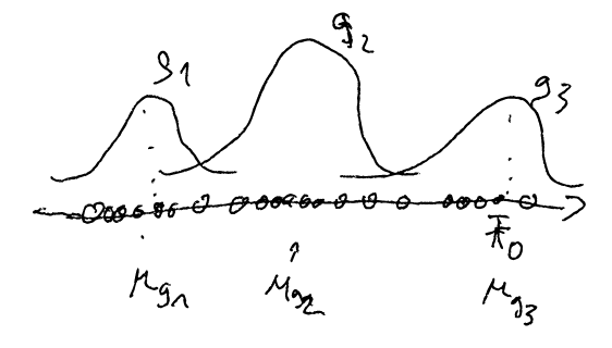
Gaussian mixture models model one distribution of each feature by a mix of several Gaussians, hence their name.


Fig.: A Gaussian mixture model for one feature (mean F0) represented by three Gaussians

(Naive) Bayes

Bayes statistics is fundamentally different from so-called frequentist statistics, as it takes prior knowledge of the problem into account.
The Bayesian formula tells us how likely an event (the class we want to distinguish) can happen in conjunction with another event (the feature that we observe).
During training the Bayes classifier updates its believe about the world, using absolute or estimated frequencies as prior knowledge.
The approach is called naive because it assumes that each input feature is independent, which is most of the time not true.


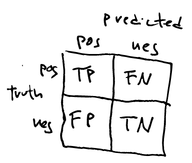
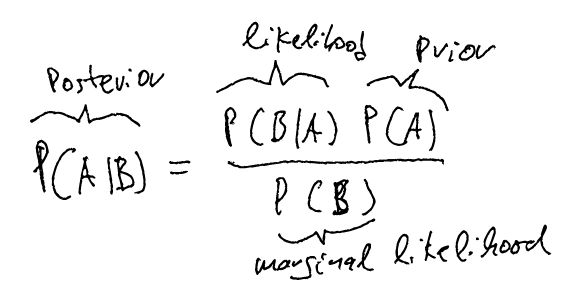
Fig.: Bayes formular predicts the occurence of some event A, given B by the co-occurence of B, given A (learned), normalized by the independent probabilities of A and B.

KNN (k nearest neighbor)

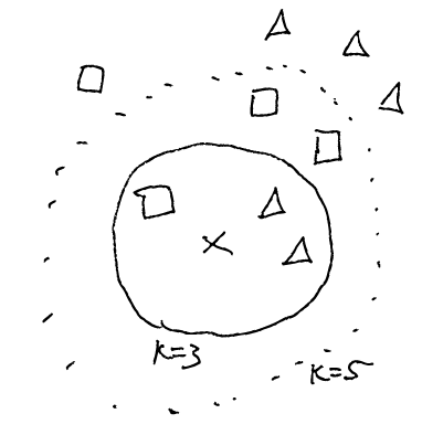
K nearest neighbor is an approach to assign test data, given its k (given parameter) nearest neighbors (in the feature space, by some distance metrics) either the most common class or some property value as an average.


Fig.: Different results for x if k=3 or k=5

Support vector machines

Support vector machines are algorithms motivated by vector geometry
They construct hyperplanes in N-dimensional (number of features) space by maximizing the margin between data points from different classes.
The function that defines the hyperplane is called the kernel function and can be parameterized.
They can be combined with GMMS if the data is approximated by them.


Fig.: A two-dimensional hyper-plane separates two classes, defined by support vectors.

CART (classification and regression trees)

Perhaps the most straightforward way to categorize data: order its parameters in a tree like fashion with the features as twigs and the data points as leaves.
The tree is learned from the training set (and can be probabilistic).
The big advantage of this model is that it is easily interpretable to humans.


Fig.: A tree predicts an emotion category for some input based on mean F0, speech rate (SR) and Harmonic-to-noise ratio (HNR)

XGBoost

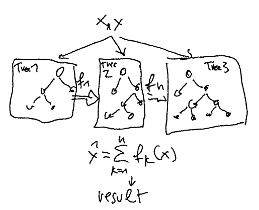
A sophisticated algorithm loosely based on CARTS as it combines Random Forests (ensembles of trees) with boosting more successful ones.


Fig.: XG boost as a result of trees, weighted by functions.

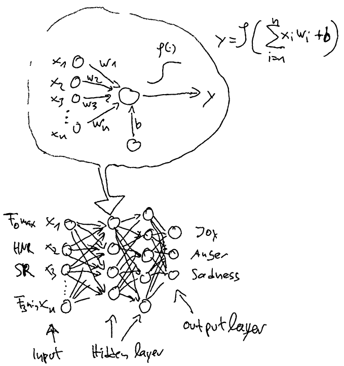
MLP (Multi-layer perceptron)

As the name suggests, these algorithms are derived from the original Perceptron idea that is inspired by the human brain.


Fig.: A feed forward network consisting of layers of Perceptrons, again predicting basic emotions for some input based on utterance global acoustic values.

Deep learning

Concepts for deep learning are discussed here