Category Archives: code

Use python for image generation

Here are some suggestions to visualize your results with python.
The idea is mainly to put your data in a pandas dataframe and then use pandas methods to plot it.

Bar plots

Here's the simple one with one variable:

vals = {'24 layers':9.37, '6 layers teached':9.94, '6 layers':10.20, 'human':10.34}
df_plot = pd.DataFrame(vals, index=[0])
ax = df_plot.plot(kind='bar')
ax.set_ylim(8, 12)
ax.set_title('error in MAE')

Here's an example for a barplot with two variables and three features:

vals_arou  = [3.2, 3.6]
vals_val  = [-1.2, -0.4]
vals_dom  = [2.6, 3.2]
cols = ['orig','scrambled']
plot = pd.DataFrame(columns = cols)
plot.loc['arousal'] = vals_arou
plot.loc['valence'] = vals_val
plot.loc['dominance'] = vals_dom
ax = plot.plot(kind='bar', rot=0)
ax.set_ylim(-1.8, 3.7)
# this displays the actual values
for container in ax.containers:
    ax.bar_label(container)

Stacked barplots

Here's an example using seaborn package for stacked barplots:
For a pandas dataframe with columns age in years and db for two database names:

import seaborn as sns
f = plt.figure(figsize=(7,5))
ax = f.add_subplot(1,1,1)
sns.histplot(data=df, ax = ax, stat="count", multiple="stack",
             x="duration", kde=False,
              hue="db",
             element="bars", legend=True)
ax.set_title("Age distriubution")
ax.set_xlabel("Age")
ax.set_ylabel("Count")

Box plots

Here's a code comparing two box plots with data dots

import seaborn as sns
import pandas as pd
n = [0.375, 0.389, 0.38, 0.346, 0.373, 0.335, 0.337, 0.363, 0.338, 0.339]
e = [0.433 0.451, 0.462, 0.464, 0.455, 0.456, 0.464, 0.461 0.457, 0.456]
data = pd.DataFrame({'simple':n, 'with soft labels':e})
sns.boxplot(data = data)
sns.swarmplot(data=data, color='.25', size=1)

Confusion matrix

We can simply use the audplot package

from audplot import confusion_matrix

truth = [0, 1, 1, 1, 2, 2, 2] * 1000
prediction = [0, 1, 2, 2, 0, 0, 2] * 1000
confusion_matrix(truth, prediction)

Pie plot

Here is an example for a pie plot

import pandas as pd

label=lst:code_fig_pie]
import pandas as pd
plot_df = 
    pd.DataFrame({'cases':[461, 85, 250]}, 
    index=['unknown', 'Corona positive', 
    'Corona negative'])
plot_df.plot(kind='pie', y='cases', autopct='%.2f')

looks like this:

Histogram

import matplotlib.pyplot as plt
# assuming you have two dataframes with a speaker column, you could plot the histogram of samples per speaker like this 
test = df_test.speaker.value_counts()[df_test.speaker.value_counts()>0]
train = df_train.speaker.value_counts()[df_train.speaker.value_counts()>0]

plt.hist([train, test], bins = np.linspace(0, 500, 100), label=['train', 'test'])
plt.legend(loc='upper right')
# better use EPS for publication as it's vector graphics (and scales)
plt.savefig('sample_dist.eps')

How to speech synthesize in German with ESPnet

Here is how to text to speech (TTS) synthesize with a German single female speaker Tacotron2 model and esp2 net

You need the python packages

pip install torch espnet_model_zoo phonemizer

Then you can run

import soundfile
from espnet2.bin.tts_inference import Text2Speech

model = 'https://zenodo.org/record/5150957/files/tts_train_tacotron2_raw_hokuspokus_phn_espeak_ng_german_train.loss.ave.zip?download=1'
text2speech = Text2Speech.from_pretrained(model)

speech = text2speech("Wow, das war ja einfach!")["wav"]
soundfile.write("out.wav", speech.numpy(), text2speech.fs, "PCM_16")

How to segment and label a speech database

Segmenting means in this case: splitting a longer audio file based on speech pauses.

This post shows you how to record, segment and then label a speech recording using the Ina speech segmenter and Labeltool.

Record audio

Firstly you need a recording. You might do that with your mobile phone or a microphone connected to your computer using, for example, Audacity.

I'd recommend recording / changing the sample rate to 16 kHz, as this is sufficient for speech recordings.

Let's say you stored your recording in the file longer_test.wav inside a directory named utterances.

Segment the recording

We start doing the segmentation in a python script.
You need some packages installed: pandas, inaSpeechSegmenter and audformat

# we start with the imports
import pandas as pd
from inaSpeechSegmenter import Segmenter
from inaSpeechSegmenter.export_funcs import seg2csv, seg2textgrid
from audformat.utils import to_filewise_index
from audformat import segmented_index

# we then use variables for our recording:
root =  './utterance/'
media = 'longer_test.wav'

# the INA speech segmenter is used very easy:
seg = Segmenter()
segmentation = seg(root+media)

# if curious, try:
print(segmentation)

# then collect the segments that were recognized as human, either female or male:
files, starts, ends = [], [], []
for entry in segmentation:
    kind = entry[0]
    start = entry[1]
    end = entry[2]
    if kind == 'female' or kind == 'male':
        print (f'{media}, {start}, {end}')
        files.append(media)
        starts.append(start)
        ends.append(end)
seg_index = segmented_index(files, starts, ends)

#  this index can now be used by audformat to acutally cut the audio file into segments
df = pd.DataFrame(index = seg_index)
file_list = to_filewise_index(df , root, 'audio_out', progress_bar = True)

# the resulting list can be stored to disk:
file_list.to_csv('file_list.csv', header=False)

Label the recording

labeling means to add metadata to the samples, for example emotional arousal.
There are hundreds of tools to do this, I use of course the one i programmed myself, Speechalyzer 😉
Here's a tutorial how to set this up and how to adapt the tool

If running on linux, you could then start the Speechalyzer with the file list you created like this:

java -jar ~/research/Speechalyzer/Speechalyzer.jar -cf ~/research/Speechalyzer/res/speechalyzer.properties -fl file_list.csv

and then simply start the Labeltool to label the files.

Speechalyzer can then export the labels to a file which can be used by Nkululeko as a labeled speech database in CSV format.

Nkululeko: meta parameter optimization

With linear classifiers that are derived from sklearn, you can simply state your variants for a meta parameter in the ini file:

[MODEL]
type = svm
tuning_params = ['C']
scoring = recall_macro
C = [10, 1, 0.1, 0.01, 0.001, 0.0001]

This will iterate the C parameter of the SVM classifier by the stated values and choose the best performing model.
You can have several "tuning_params" and them a grid search (combining everything with each other) will be performed.

Here's an example for XGB classifier:

[MODEL]
type = xgb
tuning_params = ['subsample', 'n_estimators', 'max_depth']
subsample = [.5, .7]
n_estimators = [50, 80, 200]
max_depth = [1, 6]

Here's one idea how to find the optimal values for 2 layers of an MLP net with nkululeko:

  • store your meta-parameters in arrays
  • loop over them and initialize an experiment each time
  • keep the experiment name but change your parameters and the plot name
  • this way you can re-use your extracted features and do not get your harddisk cluttered.

Here's some python code to illustrate this idea:

def main(config_file):
    # load one configuration per experiment
    config = configparser.ConfigParser()
    config.read(config_file)
    util = Util()
    l1s = [32, 64, 128]
    l2s = [16, 32, 64]
    for l1 in l1s:
        for l2 in l2s:
            # create a new experiment
            expr = exp.Experiment(config)

            plotname = f'{util.get_exp_name()}_{l1}_{l2}'
            util.set_config_val('PLOT', 'name', plotname)

            print(f'running {expr.name} with layers {l1} and {l2}')

            layers = {'l1':l1, 'l2':l2}
            util.set_config_val('MODEL', 'layers', layers)

            # load the data
            expr.load_datasets()

            # split into train and test
            expr.fill_train_and_tests()
            util.debug(f'train shape : {expr.df_train.shape}, test shape:{expr.df_test.shape}')

            # extract features
            expr.extract_feats()
            util.debug(f'train feats shape : {expr.feats_train.df.shape}, test feats shape:{expr.feats_test.df.shape}')

            # initialize a run manager
            expr.init_runmanager()

            # run the experiment
            expr.run()

    print('DONE')

Keep in mind though that meta parameter optimization like done here is in itself a learning problem. It is usually not feasible to systematically try out all combinations of possible values and thus some kind of stochastic approach is preferable.

How to set up your first nkululeko project

Nkululeko is a framework to build machine learning models that recognize speaker characteristics on a very high level of abstraction (i.e. starting without programming experience).

This post is meant to help you with setting up your first experiment, based on the Berlin Emodb.

1) Set up python

It's written in python so first you have to set up a Python environment

2) Get a database

Load the Berlin emodb database to some location on you harddrive, as discussed in this post. I will refer to the location as "emodb root" from now on.

3) Install nkululeko

Inside your virtual environment, run

pip install nkululeko

This should install nkululeko and all required modules.
It takes a long time and a lot of space, when done intially.

5) Adapt the ini file

Use your favourite editor, e.g. visual studio code and edit the file that defines your experiment. You might start with this demo sample.
You can find more templates to start here and an overview on all the options you can set here

Put the emodb root folder as the emodb value, for me this looks like this

emodb = /home/felix/data/audb/emodb

An overview on all nkululeko options should be here

6) Run the experiment

Inside a shell type (or use VSC) and start the process with

python -m nkululeko.nkululeko --config exp_emodb.ini

7) Inspect the results

If all goes well, the program should start by extracting opensmile features, and, if you're done, you should be able to inspect the results in the folder named like the experiment: exp_emodb.
There should be a subfolder with a confusion matrix named images` and a subfolder for the textual results named `results.

What to do next?

You might be interested in the hello world of nkululeko

.

Get all information from emodb

When you load the Berlin emodb as has been done in numerous postings of this blog, you will get per default only information on file name, speaker id, text id and emotion.

But there is more information contained in the audformat file and this posts shows you how to access it.

If not already somewhere on your computer, start by downloading the emodb:

if not os.path.isdir('./emodb/'):
    !wget -c https://tubcloud.tu-berlin.de/s/LfkysdXJfiobiEG
    !mv download emodb_audformat.zip
    !unzip emodb_audformat.zip
    !rm emodb_audformat.zip

This code will then load the database, prepare a single dataframe with all information and store it to disk for later use:

# load the database to memory
root = './emodb/'
db = audformat.Database.load(root)
# map the file pathes to the audio
db.map_files(lambda x: os.path.join(root, x))   
# access speaker gender and age, and transcription, from the speaker dictionaries
df = db.tables['files'].get(map={'speaker': ['speaker', 'gender', 'age'], 'transcription': ['transcription']})
# copy the emotion label from the the emotion dataframe to the files dataframe
df['emotion'] = db.tables['emotion'].df['emotion']
# add a column with the word count
df['wordcount'] = df['transcription'].apply (lambda row: len(row.split()))
# store to disk for later use
df.to_pickle('store/emodb.pkl')

df.head(1)

Machine learning experiment framework

Currently i'm working on (yet another) framework for machine learning, i.e. a python coded set of classes that can be used to run machine learning experiments in a flexible but reusable way.

I'm not sure where this is heading yet, but a first runnable version exists, if interested check it out at my github account, I'll update news there.

The general idea looks something like this:

Predict emodb emotions with a Multi Layer Perceptron ANN

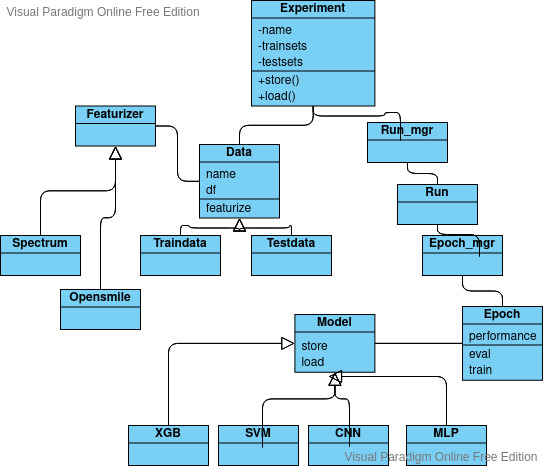
This post shows you how to classify emotions with a Multi Layer Perceptron (MLP) artificial neural net based on the torch framework (a different very famous ANN framework would be Keras).

Here's a complete jupyter notebook for your convenience.

We start with some imports, you need to install these packages, e.g. with pip, before you run this code:

import audformat
import numpy as np
import pandas as pd
import matplotlib.pyplot as plt
import torch
import os
import opensmile
from sklearn.preprocessing import LabelEncoder
from sklearn.preprocessing import StandardScaler
from sklearn.metrics import recall_score

Then we need to download and prepare our sample dataset, the Berlin emodb:

# get and unpack the Berlin Emodb emotional database if not already there
if not os.path.isdir('./emodb/'):
    !wget -c https://tubcloud.tu-berlin.de/s/8Td8kf8NXpD9aKM/download
    !mv download emodb_audformat.zip
    !unzip emodb_audformat.zip
    !rm emodb_audformat.zip
# prepare the dataframe
db = audformat.Database.load('./emodb')
root = './emodb/'
db.map_files(lambda x: os.path.join(root, x))    
df_emotion = db.tables['emotion'].df
df = db.tables['files'].df
# copy the emotion label from the the emotion dataframe to the files dataframe
df['emotion'] = df_emotion['emotion']

As neural nets can only deal with numbers, we need to encode the target emotion labels with numbers:

# Encode the emotion words as numbers and use this as target 
target = 'enc_emo'
encoder = LabelEncoder()
encoder.fit(df['emotion'])
df[target] = encoder.transform(df['emotion'])

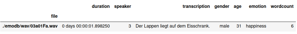
Now the dataframe should look like this:

df.head()

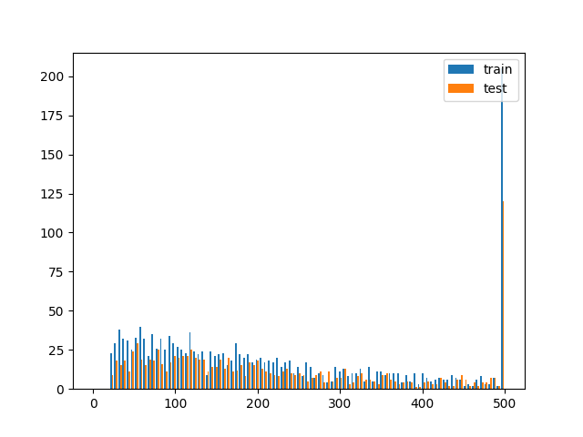
To ensure that we learn about emotions and not speaker idiosyncrasies we need to have speaker disjunct training and development sets:

# define fixed speaker disjunct train and test sets
train_spkrs = df.speaker.unique()[5:]
test_spkrs = df.speaker.unique()[:5]
df_train = df[df.speaker.isin(train_spkrs)]
df_test = df[df.speaker.isin(test_spkrs)]

print(f'#train samples: {df_train.shape[0]}, #test samples: {df_test.shape[0]}')
#train samples: 292, #test samples: 243

Next, we need to extract some acoustic features:

# extract (or get) GeMAPS features
if os.path.isfile('feats_train.pkl'):
    feats_train = pd.read_pickle('feats_train.pkl')
    feats_test = pd.read_pickle('feats_test.pkl')
else:
    smile = opensmile.Smile(
        feature_set=opensmile.FeatureSet.GeMAPSv01b,
        feature_level=opensmile.FeatureLevel.Functionals,
    )
    feats_train = smile.process_files(df_train.index)
    feats_test = smile.process_files(df_test.index)
    feats_train.to_pickle('feats_train.pkl')
    feats_test.to_pickle('feats_test.pkl')

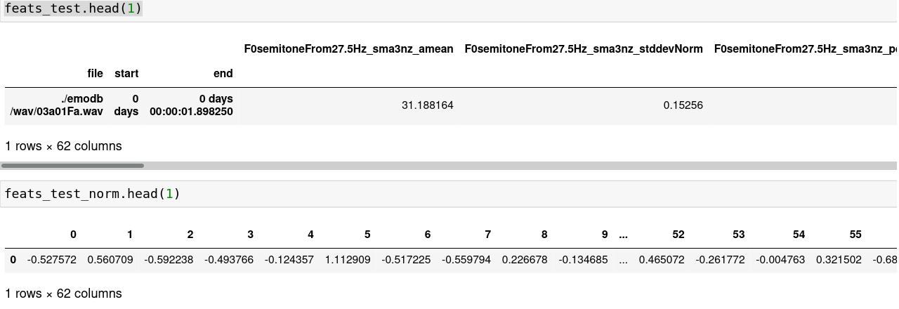
Because neural nets are sensitive to large numbers, we need to scale all features with a mean of 0 and stddev of 1:

# Perform a standard scaling / z-transformation on the features (mean=0, std=1)
scaler = StandardScaler()
scaler.fit(feats_train)
feats_train_norm = pd.DataFrame(scaler.transform(feats_train))
feats_test_norm = pd.DataFrame(scaler.transform(feats_test))

Next we define two torch dataloaders, one for the training and one for the dev set:

def get_loader(df_x, df_y):
    data=[]
    for i in range(len(df_x)):
       data.append([df_x.values[i], df_y[target][i]])
    return torch.utils.data.DataLoader(data, shuffle=True, batch_size=8)
trainloader = get_loader(feats_train_norm, df_train)
testloader = get_loader(feats_test_norm, df_test)

We can then define the model, in this example with one hidden layer of 16 neurons:

class MLP(torch.nn.Module):
    def __init__(self):
        super().__init__()
        self.linear = torch.nn.Sequential(
            torch.nn.Linear(feats_train_norm.shape[1], 16),
            torch.nn.ReLU(),
            torch.nn.Linear(16, len(encoder.classes_))
        )
    def forward(self, x):
        # x: (batch_size, channels, samples)
        x = x.squeeze(dim=1)
        return self.linear(x)

We define two functions to train and evaluate the model:

def train_epoch(model, loader, device, optimizer, criterion):
    model.train()
    losses = []
    for features, labels in loader:
        logits = model(features.to(device))
        loss = criterion(logits, labels.to(device))
        losses.append(loss.item())
        optimizer.zero_grad()
        loss.backward()
        optimizer.step()
    return (np.asarray(losses)).mean()

def evaluate_model(model, loader, device, encoder):
    logits = torch.zeros(len(loader.dataset), len(encoder.classes_))
    targets = torch.zeros(len(loader.dataset))
    model.eval()
    with torch.no_grad():
        for index, (features, labels) in enumerate(loader):
            start_index = index * loader.batch_size
            end_index = (index + 1) * loader.batch_size
            if end_index > len(loader.dataset):
                end_index = len(loader.dataset)
            logits[start_index:end_index, :] = model(features.to(device))
            targets[start_index:end_index] = labels

    predictions = logits.argmax(dim=1)
    uar = recall_score(targets.numpy(), predictions.numpy(), average='macro')
    return uar, targets, predictions

Next we initialize the model and set the loss function (criterion) and optimizer:

device = 'cpu'
model = MLP().to(device)
criterion = torch.nn.CrossEntropyLoss()
optimizer = torch.optim.Adam(model.parameters(), lr=0.0001)
epoch_num = 250
uars_train = []
uars_dev = []
losses = []

We can then do the training loop over the epochs:

for epoch in range(0, epoch_num):
    loss = train_epoch(model, trainloader, device, optimizer, criterion)
    losses.append(loss)
    acc_train = evaluate_model(model, trainloader, device, encoder)[0]
    uars_train.append(acc_train)
    acc_dev, truths, preds = evaluate_model(model, testloader, device, encoder)
    uars_dev.append(acc_dev)
# scale the losses so they fit on the picture
losses = np.asarray(losses)/2

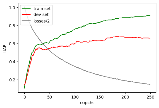
Next we might want to take a look at how the net performed with respect to unweighted average recall (UAR):

plt.figure(dpi=200)
plt.plot(uars_train, 'green', label='train set') 
plt.plot(uars_dev, 'red', label='dev set')
plt.plot(losses, 'grey', label='losses/2')
plt.xlabel('eopchs')
plt.ylabel('UAR')
plt.legend()
plt.show()

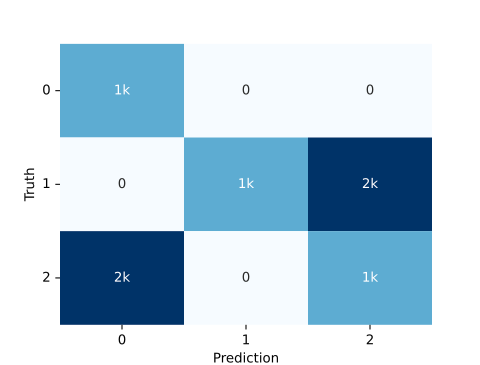
And perhaps see the resulting confusion matrix:

from sklearn.metrics import ConfusionMatrixDisplay
from sklearn.metrics import confusion_matrix
cm = confusion_matrix(truths, preds,  normalize = 'true')
disp = ConfusionMatrixDisplay(confusion_matrix=cm, display_labels=encoder.classes_).plot(cmap='gray')

Make a t-SNE plot

This post shows you how to generate a t-distributed stochastic neighbor embedding (t-SNE) plot with the opensmile features extracted from emodb data (which is explained in more detail in a previous blog post).

A t-SNE plot is a very useful visualization, as it condenses your feature space into two dimensions (so it can be plotted) and then uses colors to represent the class membership. This means, if you can identify clusters of same colored dots in your data cloud, the features are able to separate the classes.

We need the following imports:

import audformat
from sklearn.manifold import TSNE
import numpy as np
import pandas as pd
import seaborn as sns
import matplotlib.pyplot as plt
import os
import opensmile

First, you download and prepare emodb:

# get and unpack the berlin Emodb emotional database
!wget -c https://tubcloud.tu-berlin.de/s/LzPWz83Fjneb6SP/download
!mv download emodb_audformat.zip
!unzip emodb_audformat.zip
!rm emodb_audformat.zip
# preapare the dataframe
db = audformat.Database.load('./emodb')
root = './emodb/'
db.map_files(lambda x: os.path.join(root, x))
df = db.tables['emotion'].df

Then, you extract the geMAPS features:

smile = opensmile.Smile(
    feature_set=opensmile.FeatureSet.GeMAPSv01b,
    feature_level=opensmile.FeatureLevel.Functionals,
)
feats_df = smile.process_files(df.index)

And finally, you generate the t-SNE plot with the sklearn library like this:

# Plot a TSNE
def plotTsne(feats, labels, perplexity=30, learning_rate=200):
    model = TSNE(n_components=2, random_state=0, perplexity=perplexity, learning_rate=learning_rate)
    tsne_data = model.fit_transform(feats)
    tsne_data_labs = np.vstack((tsne_data.T, labels)).T
    tsne_df = pd.DataFrame(data=tsne_data_labs, columns=('Dim_1', 'Dim_2', 'label'))
    sns.FacetGrid(tsne_df, hue='label', size=6).map(plt.scatter, 'Dim_1', 'Dim_2').add_legend()
    plt.show()
plotTsne(feats_df, df['emotion'], 30, 200)

It seems that these features are useful to distinguish at least the category anger from the rest.

You might want to fiddle around with the two main parameters of the algorithm: perplexity and learning-rate.