There is a multitude of ways to model emotions, and some of them are collected in the EmotionML vacabularies.
Really popular with engineers and non-psychologists are two approaches:

• discreet categories like anger, sadness, fear or joy, often associated with an intensity.
• continuous dimensions like valence/pleasure, arousal or dominance

The emotion cube maps the emotional categories to a three dimensional space:

In supervised machine learning, you usually need three kinds of data sets:

• train data: to teach the model the relation between data and labels
• dev data: (short for development) to tune meta parameters of your model, e.g. number of neurons, batch size or learning rate.
• test data: to evaluate your model ONCE at the end to check on generalization

Of course all this is to prevent overfitting on your train and/or dev data.

If you've used your test data for a while, you might need to find a new set, as chances are high that you overfitted on your test during experiments.

So what's a good split?

Some rules apply:

• train and dev can be from the same set, but the test set is ideally from a different database.
• if you don't have so much data, a 80/20/20 % split is normal
• if you have masses an data, use only so much dev and test that your population seems covered.
• If you have really little data: use x cross validation for train and dev, still the test set should be extra

Nkululeko exercise

Edit the demo configuration

1)
Set/keep as target emotion as FEAT type os and as MODEL type xgb

Use the emodb as test and train set but try out all split methods

• specified
• speaker split
• random
• loso
• logo
• 5_fold_cross_validation

Which works best and why?

2)
Set the

[EXP]
epochs = 200
[MODEL] 
type = mlp
layers = {'l1':1024, 'l2':64} 
save = True
[PLOT]
epoch_progression = True
best_model = True

run the experiment.
Find the epoch progression plot and see at which epoch overfitting starts.

This post is about evaluation of machine learning models, obviously the answer to the question if a model is any good depends a lot on how you test that.

Criteria

Depending whether you got a classification or regression problem you can choose from a multitude of measures.

Classification

Most of these are derived from the confusion matrix:

• Confusion Matrix : Matrix with results: rows represent the real values and columns the predictions. In the binary case, the cells are called True Positive (TP), False Negative (FN: Type 2 error), False Positive (FN: Type 1 error) and True Negative (TN)
  Here's a plot of cases: idea
  
  In this figure, the circles are the relevant samples and the crosses are the not-relevant ones. Now the relevant ones that are not in the selected area are False Negatives, and the ones inside are True Positive.

And this would be the confusion matrix:

So in the example above, TP=3, FN=4, FP=3 and TN=3.

The following measurements can be derived from these:

• Accuracy: Percentage of correct predictions -> (TP+TN)/(TP+FP+FN+TN).

• un- / weighted Recall/Sensitivity: percentage of detected cases -> TP / (TP+FN). Can be weighted by class frequency, for multiple classes

• un- / weighted Precision: percentage of relevant predictions -> TP / (TP+FP)

• Specificity: Like sensitivity, but for the negative examples -> TN / (TN+FP)

• F1: Combination of Recall and Precision -> F1 = 2 (Rec Prec)/ (Rec + Prec)

• AUC/ROC Usually there's a tradeoff between Recall and Precision. With the Receiver Operator Curve and it's Area under curve this can be visualized by plotting the False positive rate (100-specificity) against the True positive rate (sensitivity).

  Regression

• Pearson's Pearson's Correlation Coefficient measures the similarity of two sets of numbers with the same lenght. I's a value between -1 and 1, with 0 meaning no correlation and -1 negative correlation. When plotted in 2-d space, PCC=1 would be the identity line.

• MAE Mean absolute error: taken two sets of numbers with same length as correct and predicted values, one can compute the mean absolute error by summing up the absolute values of the pairwise differences and scale by the number of samples.

• CCC Concordance Correlation Coefficient is a measure quite similar to PCC but tries to penalize rater bias (seeing the two distributions as truth and ratings).

Approaches

Train / test /dev splits

Best you have enough data to split it into seperate sets:

• train for the training
• dev to tune meta-parameters
• test as a final test set

Be careful to make sure that they are speaker disjunct, i.e. not have overlapping speakers, else you can't be sure if you learn general speaker characteristics or speaker idiosyncrasies.

Also it's a very good idea to have the test set from a completely different data source, so you could have more trust in the generalizability of your model.

More on the subject here

X fold cross validation

If you are low on data, you might try x fold cross validation, it means that you split your data in x (usually 10) sets with same size, and then do x trainings, using one set as dev set and the rest for train.

LOSO

Leave one Speaker out is like X fold cross-validation, but each set are all samples of one speaker. If there are many speakers, you might want Leave one speaker group out.
Both is supported by Nkululeko.

This post gives an overview on popular machine learners in a nutshell.
Lots of site on the internet give great detail on this and you should take a few minuted to check them out.

Preliminaries and some naming conventions

In general, all these approaches work by extracting features from data and comparing a test sample's features with the features derived from a training set to predict some class or value in case of regression.

So they work with two phases:

• During training, the parameters of the approach are learned, thereby creating the model.
• A test time, unknown test samples get predicted by the model.

In addition, most of these approaches can be customized by meta-parameters which also can be learned by some meta algorithm, but not during a normal training.

One thing all of these approaches have in common is that they model the world by "densing" down the real values, i.e. the data, to a simpler form at some time (feature extraction), so they all can be seen as some kind of dimensionality reduction

On the one hand you lose information this way, on the other this is not a problem because you usually are interested in some kind of underlying principle that generated your training data, and not so much in the training data itself.
Still you got a trade-off between generality and specificity

Obviously, the following list is by far not complete, I simply selected the ones that were most commonly used during my professional life.

Linear regression

To represent the dependency of a dependend and an independend variable by a straight line. The price question is how to learn the two parameters of the line (a and b of y=ax+b) using the training data. One approach would be gradient descent with a Perceptron.

Fig.: Two linear regression models for anger and happiness based on mean fundamental frequency (F0)

GMMs

A Gaussian is a way to describe a distribution with two values: mean and variance. Now one way to distinguish two kinds of things is two distinguish them by the distributions of their features, e.g. herrings from trouts by the size of their fins.
Gaussian mixture models model one distribution of each feature by a mix of several Gaussians, hence their name.

Fig.: A Gaussian mixture model for one feature (mean F0) represented by three Gaussians

(Naive) Bayes

Bayes statistics is fundamentally different from so-called frequentist statistics, as it takes prior knowledge of the problem into account.
The Bayesian formula tells us how likely an event (the class we want to distinguish) can happen in conjunction with another event (the feature that we observe).
During training the Bayes classifier updates its believe about the world, using absolute or estimated frequencies as prior knowledge.
The approach is called naive because it assumes that each input feature is independent, which is most of the time not true.

Fig.: Bayes formular predicts the occurence of some event A, given B by the co-occurence of B, given A (learned), normalized by the independent probabilities of A and B.

KNN (k nearest neighbor)

K nearest neighbor is an approach to assign test data, given its k (given parameter) nearest neighbors (in the feature space, by some distance metrics) either the most common class or some property value as an average.

Fig.: Different results for x if k=3 or k=5

Support vector machines

Support vector machines are algorithms motivated by vector geometry
They construct hyperplanes in N-dimensional (number of features) space by maximizing the margin between data points from different classes.
The function that defines the hyperplane is called the kernel function and can be parameterized.
They can be combined with GMMS if the data is approximated by them.

Fig.: A two-dimensional hyper-plane separates two classes, defined by support vectors.

CART (classification and regression trees)

Perhaps the most straightforward way to categorize data: order its parameters in a tree like fashion with the features as twigs and the data points as leaves.
The tree is learned from the training set (and can be probabilistic).
The big advantage of this model is that it is easily interpretable to humans.

Fig.: A tree predicts an emotion category for some input based on mean F0, speech rate (SR) and Harmonic-to-noise ratio (HNR)

XGBoost

A sophisticated algorithm loosely based on CARTS as it combines Random Forests (ensembles of trees) with boosting more successful ones.

Fig.: XG boost as a result of trees, weighted by functions.

MLP (Multi-layer perceptron)

As the name suggests, these algorithms are derived from the original Perceptron idea that is inspired by the human brain.

Fig.: A feed forward network consisting of layers of Perceptrons, again predicting basic emotions for some input based on utterance global acoustic values.

Deep learning

Concepts for deep learning are discussed here

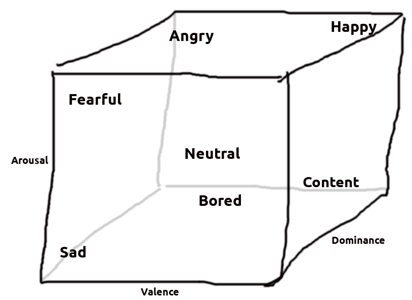
The speech AI company audEERING open sourced a model to classify emotional dimensions, i.e. arousal, valence and dominance.

In this tutorial, let's see how the open-domain emotional database EmoDB is categorized by this model (which is trained on a different emotional database: MSPPodcast).

Thanks to Johannes Wagner for providing the code used in this tutorial.

We'll do this in a jupyter notebook.
Here is the list of requirements you need to install (after having activated your environment):

pip install juypter pandas umap-learn audb audonnx matplotlib seaborn audinterface

We start our notebook with the imports:

import numpy as np
import pandas as pd
import umap
import matplotlib.pyplot as plt
import seaborn as sns
import audeer
import audonnx
import audb
import audformat
import audinterface
# and two constants:
sampling_rate = 16000
model_id = '6bc4a7fd-1.1.0'

We'll then load the model like this:

url = f'https://zenodo.org/record/6221127/files/w2v2-L-robust-12.{model_id}.zip'
cache_root = audeer.mkdir('cache')
model_root = audeer.mkdir('model')
archive_path = audeer.download_url(url, cache_root, verbose=True)
audeer.extract_archive(archive_path, model_root)
model = audonnx.load(model_root)
# and inspect it:
print(model)

We load the database:

db = audb.load(
    'emodb',
    version='1.3.0',
    format='wav',
    mixdown=True,
    sampling_rate=sampling_rate,
)
emotion_test = db[f'emotion.categories.test.gold_standard']['emotion'].get()
emotion_train = db[f'emotion.categories.train.gold_standard']['emotion'].get()
emotion = pd.concat([emotion_test, emotion_train])
speaker = db['files']['speaker'].get(emotion.index)
gender = db['files']['speaker'].get(emotion.index, map='gender')
transcription = db['files']['transcription'].get(emotion.index)
df_labels = audformat.utils.concat([emotion, speaker, gender, transcription])
df_labels.head(1)
print(df_labels.shape)

We create two interface: one for the logits (emotional dimensions) and one for the features (embeddings: pen-ultimate layer of network).

interface_logits = audinterface.Feature(
    model.labels('logits'),       # feature names
    process_func=model,
    process_func_args={
        'outputs': 'logits',      # output 'logits'
    },   
    verbose=True,
)
interface_features = audinterface.Feature(
    model.labels('hidden_states'),
    process_func=model,
    process_func_args={
        'outputs': 'hidden_states',
    },
    verbose=True,
)

and then we can extract them simply by stating:

df_features = interface_features.process_index(
    df_labels.index, 
    cache_root=audeer.path(cache_root, model_id, 'features'),
)
df_logits = interface_logits.process_index(
    df_labels.index, 
    cache_root=audeer.path(cache_root, model_id, 'logits'),
)
# and inspect them
print(df_logits.head(1))
print(df_logits.shape, df_features.shape)

To visualize, we transform the features to two dimensions:

y_umap = umap.UMAP(
    n_neighbors=10,
    random_state=0,
).fit_transform(df_features.values)

pd.DataFrame(
    y_umap,
    df_features.index,
    columns=['umap-0', 'umap-1'],
)

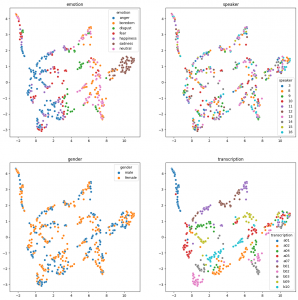
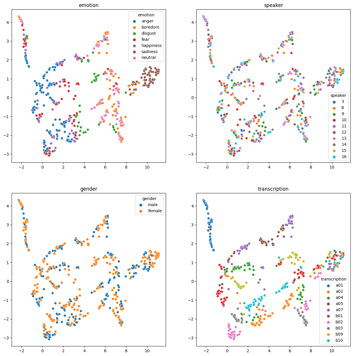
And then plot these, colored by the labels of the database:

fig, axs = plt.subplots(2, 2, figsize=[15, 15])
axs = axs.flatten()

for ax, column in zip(axs, df_labels):
    ax.set_title(column)
    _ = sns.scatterplot(
        x=y_umap[:, 0],
        y=y_umap[:, 1],
        hue=df_labels[column],
        ax=ax,
    )

Which should leave you with:

A great read as an introduction to emotional speech is Marc Schröder's first chapters of his dissertation which is available online at the university of Saarland